Step 4: Output and visualisation • biomes

Goal

The records were assigned to biome classes in Step 3. This final step summarises the result per biome class with biomes_tab() and visualises the whole workflow with biomes_visualise().

1. Tabulate records per biome class

biomes_tab() counts occurrence records (one input row = one record) per biome class and scheme, returning a long table with one row per (scheme, biome class) pair:

classified <- biomes_classify(biomes_example, scheme = 1)
#> Coordinates provided as data.frame, assuming WGS84 as CRS.
#> Classified 29104 record(s) against 1 biome layer(s):
#>   - Biome_Inventory_layer_01 (Allen et al., 2020)
biomes_tab(classified)
#>                      scheme                                 biome    n
#> 1  Biome_Inventory_layer_01    Boreal evergreen needleleaf forest 2217
#> 2  Biome_Inventory_layer_01                       Boreal parkland  367
#> 3  Biome_Inventory_layer_01   Boreal summergreen broadleaf forest  384
#> 4  Biome_Inventory_layer_01                                Desert  221
#> 5  Biome_Inventory_layer_01                              no_biome 4652
#> 6  Biome_Inventory_layer_01                               Savanna  447
#> 7  Biome_Inventory_layer_01                            Semidesert  583
#> 8  Biome_Inventory_layer_01                          Shrub tundra  483
#> 9  Biome_Inventory_layer_01                                Steppe  148
#> 10 Biome_Inventory_layer_01  Temperate broadleaf evergreen forest 5171
#> 11 Biome_Inventory_layer_01                Temperate mixed forest 1687
#> 12 Biome_Inventory_layer_01 Temperate needleleaf evergreen forest  323
#> 13 Biome_Inventory_layer_01                    Temperate parkland  407
#> 14 Biome_Inventory_layer_01                   Temperate shrubland  729
#> 15 Biome_Inventory_layer_01          Temperate summergreen forest 6139
#> 16 Biome_Inventory_layer_01             Tropical evergreen forest 1860
#> 17 Biome_Inventory_layer_01                    Tropical grassland  118
#> 18 Biome_Inventory_layer_01             Tropical raingreen forest  824
#> 19 Biome_Inventory_layer_01                                Tundra    2
#> 20 Biome_Inventory_layer_01               Warm temperate woodland 2342

The returned columns are scheme, biome and n. To count unique species per biome class instead of records, deduplicate by species first:

library(dplyr)
#> 
#> Attaching package: 'dplyr'
#> The following objects are masked from 'package:terra':
#> 
#>     intersect, union
#> The following objects are masked from 'package:stats':
#> 
#>     filter, lag
#> The following objects are masked from 'package:base':
#> 
#>     intersect, setdiff, setequal, union

classified |>
  distinct(species, Biome_Inventory_layer_01_name) |>
  biomes_tab()
#>                      scheme                                 biome  n
#> 1  Biome_Inventory_layer_01    Boreal evergreen needleleaf forest  7
#> 2  Biome_Inventory_layer_01                       Boreal parkland 11
#> 3  Biome_Inventory_layer_01   Boreal summergreen broadleaf forest  5
#> 4  Biome_Inventory_layer_01                                Desert 10
#> 5  Biome_Inventory_layer_01                              no_biome 13
#> 6  Biome_Inventory_layer_01                               Savanna 17
#> 7  Biome_Inventory_layer_01                            Semidesert 12
#> 8  Biome_Inventory_layer_01                          Shrub tundra  5
#> 9  Biome_Inventory_layer_01                                Steppe 11
#> 10 Biome_Inventory_layer_01  Temperate broadleaf evergreen forest 25
#> 11 Biome_Inventory_layer_01                Temperate mixed forest 10
#> 12 Biome_Inventory_layer_01 Temperate needleleaf evergreen forest  9
#> 13 Biome_Inventory_layer_01                    Temperate parkland  7
#> 14 Biome_Inventory_layer_01                   Temperate shrubland 18
#> 15 Biome_Inventory_layer_01          Temperate summergreen forest 10
#> 16 Biome_Inventory_layer_01             Tropical evergreen forest 20
#> 17 Biome_Inventory_layer_01                    Tropical grassland 11
#> 18 Biome_Inventory_layer_01             Tropical raingreen forest 22
#> 19 Biome_Inventory_layer_01                                Tundra  1
#> 20 Biome_Inventory_layer_01               Warm temperate woodland 14

2. Visualise the workflow

biomes_visualise() draws up to three panels for a set of occurrence records:

rank: the ranking of the biome schemes (best highlighted);
map: the occurrence records (red points) over the chosen scheme, with the number of records per biome class appended to the legend labels;
barplot: the number of records and species per biome class.

By default all three are drawn and lettered a, b, c. If scheme is NULL, the best-fitting scheme is chosen by biomes_rank() (within scheme_type).

biomes_visualise(biomes_example)               # rank + map + barplot
#> <SpatRaster> resampled to 5e+05 cells.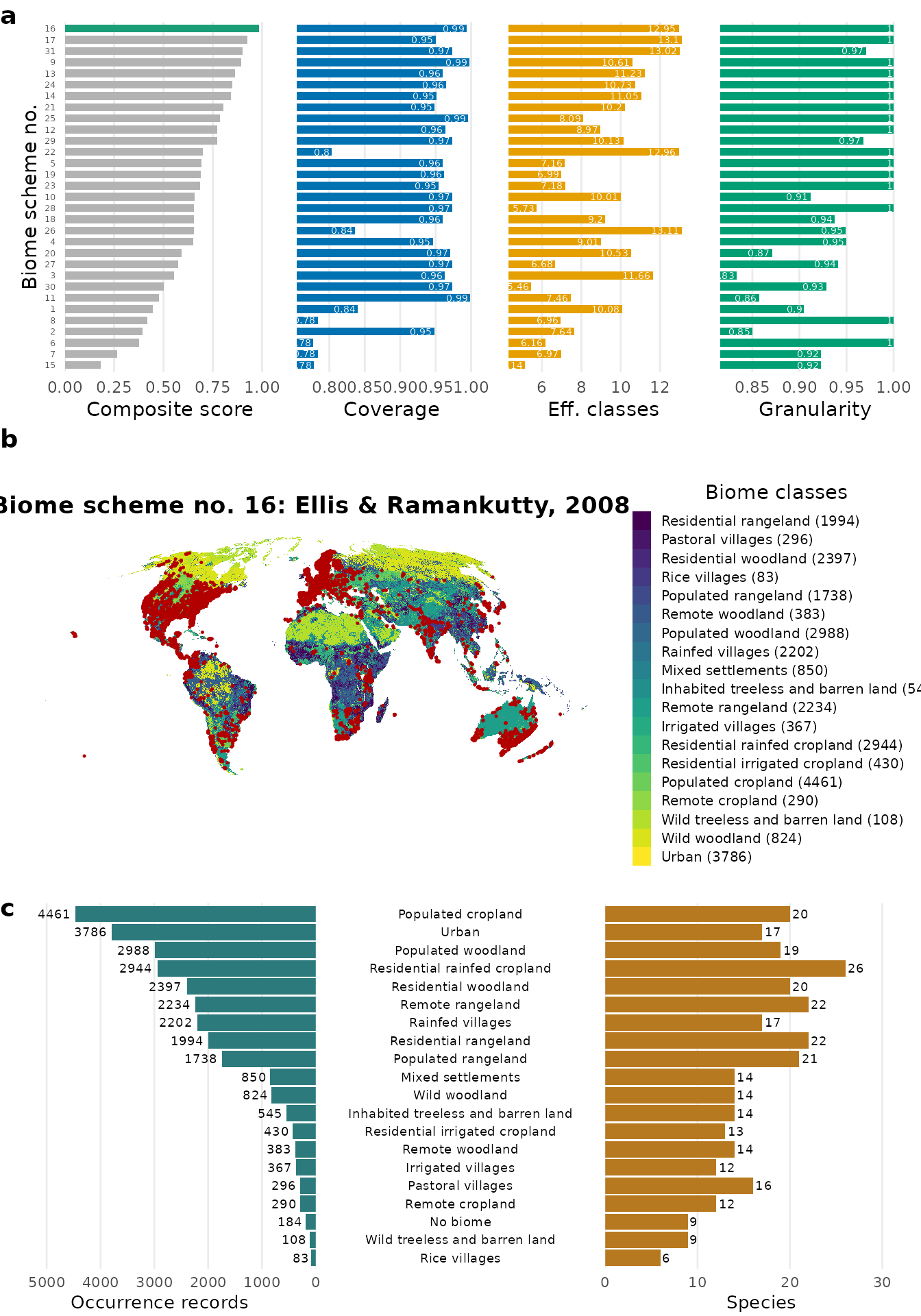

Ranking, occurrence map and biome-class composition

Select individual panels with panels; the panel letters adjust to the selection (e.g. panels = c("map", "barplot") labels them a and b):

# just the map, for a fixed scheme
biomes_visualise(biomes_example, scheme = 1, panels = "map")
#> <SpatRaster> resampled to 5e+05 cells.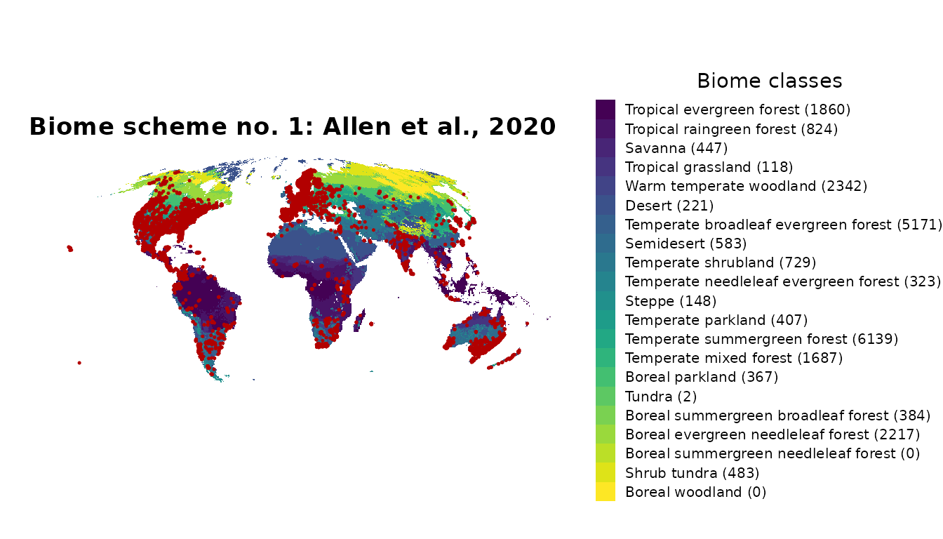

Occurrence map over biome scheme 1

The red points are the occurrence records you supplied. Drop the record counts from the legend labels with legend_counts = FALSE, or the whole colour legend with legend = FALSE. Save any panel with ggplot2::ggsave():

p <- biomes_visualise(biomes_example, scheme = 1, panels = "map", legend = FALSE)
ggplot2::ggsave("biome_map.jpg", p, width = 13, height = 8, dpi = 600)

The whole workflow in one call

Steps 1-4 are wrapped by biomes_full(), which by default ranks across all 31 schemes and uses the best one. No figure is drawn by default (plot = "none", the fastest option). plot = "all" returns the combined lettered figure in res$plot:

res <- biomes_full(x = biomes_example, plot = "all")   # scheme = "best"
res$scheme     # the chosen biome scheme number
res$table      # records per biome class
res$plot       # the combined figure (rank + map + barplot)

A subset of c("rank", "map", "barplot") returns the panels individually (no panel letters), each in its own component res$rank, res$map, res$barplot:

res <- biomes_full(x = biomes_example, plot = c("rank", "map", "barplot"))
res$map        # just the map panel, on its own
res$barplot    # just the barplot panel

To force a specific scheme, pass its number (scheme = 1); to rank within one group, pass a scheme type (scheme = "vegetation"). Reach for the individual functions when you want to tweak a step; use biomes_full() when you want the standard pipeline in one call.

Done

That completes the four-step workflow: assemble → choose a scheme → classify → output and visualise. Back to Step 1.