Step 2: Choice of a biome scheme

Goal

Step 1 gave us occurrence records and the 31 biome schemes. With 31 schemes to choose from, this step picks the one that best fits your data, so the choice is explicit and reproducible rather than defaulting to a familiar scheme.

Terms. A biome scheme is one of the 31 classification systems; a biome is a category within it; a biome scheme number (1-31) identifies a scheme. A biome definition is the concept on which a scheme delimits its biomes; the definition argument restricts the ranking to the schemes sharing one definition.

1. Rank the schemes for your data

biomes_rank() scores every scheme for your occurrences and proposes a single best-fitting scheme. Each scheme is rated on three complementary, data-driven criteria:

coverage: share of records that fall on a defined biome.
effective number of biomes: exp(H'), the effective number of biomes the records occupy (rewards schemes that spread the data over several well-populated biomes).
granularity: occupied biomes divided by the total number of biomes in the scheme.

The three criteria are min-max scaled to [0, 1] across the compared schemes and averaged (equal weights) into a composite score. The best-scoring scheme is returned in attr(ranking, "best_scheme").

Because the scaling is relative to the compared schemes, a composite score is only comparable among schemes that were ranked together, and a scaled value of 0 means “lowest among the compared schemes”, not zero. A criterion that does not vary among the compared schemes is left out of the composite (see attr(ranking, "criteria_used")), and a single compared scheme gets no composite score. Ties in the composite score are broken by the publication year of the scheme (more recent first; see tiebreaker).

ranking <- biomes_rank(bombacoideae_occurrences, verbose = FALSE)
best    <- attr(ranking, "best_scheme")
best
#> [1] 16
head(ranking)
#>   scheme
#> 1      1
#> 2      2
#> 3      3
#> 4      4
#> 5      5
#> 6      6
#>                                                                                                                  scheme_name
#> 1                                                                       Global vegetation patterns of the past 140,000 years
#> 2                                                  Dataset of the global component of the Copernicus Land Monitoring Service
#> 3                                            Present and future Köppen-Geiger climate classification maps at 1-km resolution
#> 4 Global mapping of potential natural vegetation: an assessment of machine learning algorithms for estimating land potential
#> 5                                                       An ecoregion-based approach to protecting half the terrestrial realm
#> 6                                              A global classification of vegetation based on NDVI, rainfall and temperature
#>   year n_total n_hit n_na pct_na coverage_raw coverage_scaled
#> 1 2020   17030 15999 1031   6.05    0.9394598       0.3369938
#> 2 2019   17030 16175  855   5.02    0.9497945       0.4577900
#> 3 2018   17030 16497  533   3.13    0.9687023       0.6787920
#> 4 2018   17030 16183  847   4.97    0.9502642       0.4632807
#> 5 2017   17030 16488  542   3.18    0.9681738       0.6726150
#> 6 2017   17030 15928 1102   6.47    0.9352907       0.2882636
#>   effective_biomes_raw effective_biomes_scaled granularity_raw
#> 1             4.721102              0.10251879       0.7142857
#> 2             6.556205              0.31649699       0.7500000
#> 3             5.818907              0.23052595       0.5000000
#> 4             5.324543              0.17288175       0.7000000
#> 5             4.329130              0.05681376       0.8666667
#> 6             3.841888              0.00000000       0.6428571
#>   granularity_scaled composite_score rank is_best
#> 1          0.5142857       0.3179328   28   FALSE
#> 2          0.5750000       0.4497623   19   FALSE
#> 3          0.1500000       0.3531060   25   FALSE
#> 4          0.4900000       0.3753875   23   FALSE
#> 5          0.7733333       0.5009207   16   FALSE
#> 6          0.3928571       0.2270402   31   FALSE

The result is a data frame with one row per scheme; the key columns are scheme (the biome scheme number), scheme_name, composite_score and is_best.

Rank within one biome definition

Comparing schemes built on different biome definitions can mislead, so restrict the ranking to the schemes sharing one definition with definition:

r_veg <- biomes_rank(bombacoideae_occurrences, definition = "vegetation", verbose = FALSE)
attr(r_veg, "best_scheme")
#> [1] 25

table(biomes_information$biome_definition)   # how many schemes per group
#> 
#> anthropogenic       climate     ecoregion   integrative    land_cover 
#>             1             7             4             6             7 
#>    vegetation 
#>             6

definition = "all" (the default) ranks all 31 schemes. The biome definitions are "climate", "vegetation", "land_cover", "ecoregion", "integrative" and "anthropogenic".

2. Inspect the ranking

The rank panel of biomes_visualise() shows the composite score per scheme with the best scheme highlighted:

biomes_visualise(bombacoideae_occurrences, panels = "rank")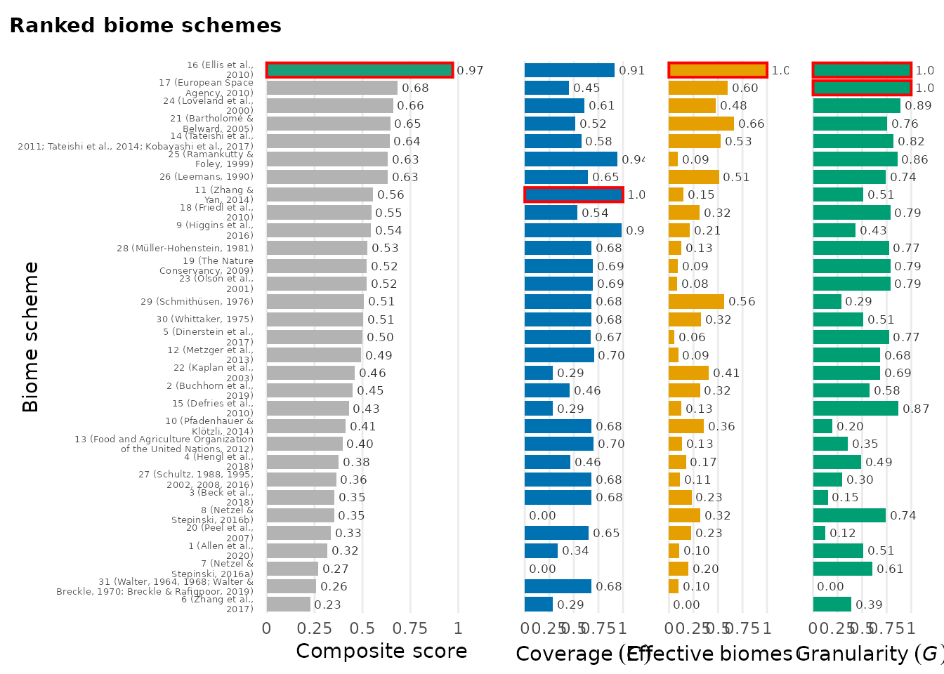

Treat the ranking as a shortlist, not an authoritative answer: the most suitable scheme ultimately depends on your research question. Inspect the criterion-specific columns of the ranking and use biomes_info() to pick the scheme whose concept and resolution match your data.

The integer in attr(ranking, "best_scheme") is exactly the biome scheme number you pass as scheme to the classification and visualisation functions next.

You have a chosen biome scheme. Continue with Step 3: Occurrences-to-biome classification.

Goal

1. Rank the schemes for your data

Rank within one biome definition

2. Inspect the ranking

Next